
406 阅读 2020-02-04 17:36:01 上传
Learning the mapping function from voltage amplitudes to sensor positions in
3D-EMA using deep neural networks
Christian Kroos, Mark D. Plumbley
Centre for Vision, Speech and Signal Processing (CVSSP)
University of Surrey
Guildford, Surrey, GU2 7XH, UK
c.kroos@surrey.ac.uk, m.plumbley@surrey.ac.uk
Abstract
The first generation of three-dimensional Electromagnetic Articulography devices (Carstens AG500) suffered from occasional critical tracking failures. Although now superseded by new devices, the AG500 is still in use in many speech labs and many valuable data sets exist. In this study we investigate whether deep neural networks (DNNs) can learn the mapping function from raw voltage amplitudes to sensor positions based on a comprehensive movement data set. This is compared to arriving sample by sample at individual position values via direct optimisation as used in previous methods. We found that with appropriate hyperparameter settings a DNN was able to approximate the mapping function with good accuracy, leading to a smaller error than the previous methods, but that the DNN-based approach was not able to solve the tracking problem completely.
Index Terms: Electromagnetic Articulography, 3D-EMA, position estimation, deep neural networks, DNN, speech articulation
1. Background
Electromagnetic Articulography (EMA) allows measuring the movements of the speech articulators in real-time without relying on a line of sight between the studied articulators and the device. Over the last decades it has become an important tool in experimental phonetics [1]. Starting out in the 1980s as limited two-dimensional system confined to the midsagittal plane, method and devices have matured over time to track simultaneously several sensors with sufficient temporal resolution and spatial accuracy. At the begin of the century the first three-dimensional system (3D-EMA) was introduced, first as prototype [2, 3], and later as a commercial system, the Carstens AG500. Currently, two commercial systems are available: the AG501 (Carstens Medizinelektronik GmbH) and the Wave System (Northern Digital, Inc.).
The systems use different device architectures and algorithms but share the underlying principle: A small sensor coil is placed in a alternating electromagnetic field created by a number of transmitter coils part of the main device. The electromagnetic field induces a very weak voltage in the sensor coils. The strength of the induced signal depends on the distance of the sensor from the transmitter and the relative orientation difference between the transmitter and sensor coil axes. With a single-axis-coil sensor only five of the six degrees of freedom can be recovered: the three location coordinates (x, y, z) and two of the three orientation parameters (azimuth, elevation). The rotation of the sensor around its own axis does not lead to a change in the induced signal and can therefore not be estimated.
The first generation of 3D-EMA devices, solely the AG500 mentioned above, had six transmitters coils mounted to a plexiglass cube at different locations and in different orientations, designed to yield an overdetermined set of equations for estimating the sensor position. Since the electromagnetic field equation contains non-linear terms and no analytic solution is known, a non-linear optimisation method has to be employed (e.g., Newton-Raphson, Levenberg-Marquardt). Despite being able to rely in general on good starting values in the form of the previous sample, the optimisation often fails to converge on the proper value. Reports on the accuracy vary slightly based on the evaluation method and error measure used [4, 5, 6, 7, 8], but all note occasionally occurring very large errors.
In previous work [6], the first author of the present paper showed that these big errors do not necessarily arise in the form of a sudden jumps. The calculated trajectories can deviate smoothly but increasingly from the true trajectories, rendering it very difficult to identify mistracking in real-world experiments. Stella et al. [7] demonstrated that the the episodes of tracking failure are largely due to numerical instabilities of the optimisation methods in certain areas of the combined locationorientation space and the more recent devices (the Wave system and the AG501) do not suffer from these shortcomings any more due to an increased number of transmitters. The AG500, however, is still in use in many research labs and valuable data set have been recorded in the past, some of them might never be recorded again (e.g., the data set used in [9]). Because of the aforementioned problems, frequently substantial portions had and have to be discarded. We deemed it therefore worthwhile to investigate whether an alternative method of determining the position data from the voltage amplitudes could mitigate the tracking problems or, ideally, completely remove them. Obviously, that latter will be only possible if they are not due to deconvolution artefacts or other system-immanent noise and are solely caused by optimisation errors. This might be indeed the case as [7] concluded.
A promising approach providing such an alternative to the commonly used direct optimisation methods is to use deep learning with artificial deep neural networks (DNNs, [10, 11], for a review see [12]) to learn the functional mapping from the data. The development history of deep neural nets goes back at least two decades but only within the last years their success in a variety of classification, detection and synthesis tasks has made them the most popular techniques in machine learning. Shallow artificial neural networks with only one hidden layer have been shown to be able to theoretically approximate any continuous function [13]. However, given complex functions the number of nodes in the hidden layer might need to be exceedingly large. It has been also shown that deep neural networks, that is, networks with many hidden layers, reduce the number of required nodes substantially [14]. Initial procedural problems of how to train these network were overcome and the necessary computational resources are now available and very large data set widespread.
In the current study, the task appears to be relatively simple, a non-linear regression requiring only a mapping from a six-dimensional input space to a five-dimensional output space. By ignoring the orientation angles, which are seldom used in speech research, the output space even reduces to three dimension. However, due to the complexity of the electromagnetic field and in particular the impact of orientation angle changes, the mapping is far from being an easy inverse problem. In addition, it is difficult to acquire a data set that approximately equally samples the entire output space, because the sensors have to be physically moved and not only the EMA measurements have to be acquired but also some kind of ground truth. Accordingly the (deep) neural net has to learn from an incomplete and potentially biased data set.

Our starting point in the current study is the dataset acquired for the evaluation of the AG500’s measurement accuracy in [6]. Serving as ground truth are recordings simultaneously acquired with a more precise, optical motion capture system (see Method section).
Our research question was whether a deep neural network (DNN) would be able to approximate the mapping function sufficiently close to produce more accurate location coordinates than achieved with the direct methods and, in particular, whether the DNN would be able to avoid the occasional large deviations seen in the direct methods. We hypothesised that (i) a DNN would be able to learn the mapping function and (ii) would be able to improve substantially on the direct methods. The criterion value for (i) was set to the root mean squared error (RMSE) value achieved by the direct methods. If the DNN would score among them or better, the hypothesis would be considered confirmed. The criterion for (ii) was set to the RMSE error value of the direct methods resulting after deviations above the Euclidean distance threshold of 10 mm were manually excluded for the direct methods (see [6]), but not the DNN.
Note that we did not intend to utilise the temporal order of the samples, despite the fact that for speech movements a high degree of smoothness can be assumed with the potential exception of trills and cases in which an articulator movement is stopped by a rigid boundary, e.g. tongue tip movements halted by the hard palate in some stop consonants (if the tongue is not gliding along the hard palate). Our aim was to examine whether the true underlying mapping function could be recovered.
2. Method
2.1. Data acquisition
As the data acquisition is described in detail in [6], we will only briefly summarise it here. We acquired a rich set of movement data with the AG500 (henceforth shortened to EMA) at the MARCS Institute (Western Sydney University, Australia) together with recordings with the optical, marker-based Vicon system (henceforth OPT). The tracking with the latter system was accomplished with eight MX-40 cameras and the manufacturer claims an accuracy of 0.1 mm. The data of the two systems were temporally aligned using a trigger signal produced by the AG500’s Sybox and spatially aligned by wrapping a set of EMA markers with reflective foil, turning them into simultaneous OPT markers. The marker-sensor combinations were spread across the measurement field in the EMA cube and a few static trials recorded.
For the movement trials the EMA sensors were fixed in a custom-build container and the OPT markers fixed to a three-dimensional cross-shaped structure attached to the container (see Figure 1). The container enabled to examine sensor orientation angles that are, of course, not returned by the OPT system, but can be computed via rigid-body pose estimation algorithms (e.g., Generalized Procrustes method [15], for use in 3D-EMA see also [16]). The container was manually moved by an experimenter. We recorded eight different sets of movements each with 40 trials: three sets with predominately translational movements along the three major coordinate axes, three with rotational movements around the major coordinate axes, one set with no motion and one set with unconstrained movements, comprising a combination of all translations and rotations. The sample rate was 200 Hz and a single trial lasted for 10 s, yielding 2000 samples.
Table 1: Number of ambiguous amplitude-position relations out of the possible total of 1.84 · 1010 .

The raw EMA data (voltages) were processed with both available routines: CalcPos from the manufacturer and TAPAD from the Phonetics Department of Munich University [17]. The locations of the EMA sensors and OPT markers relative to each other in/at the container across systems were determined by using the static trials, in which the container was motionless suspended in the cube centre, and by taking the mean coordinate differences of the centre of gravity for both systems of all static trials after spatial (and temporal) alignment of the coordinate systems described above. Subsequently, the locations and orientation of the EMA sensors were sample-wise predicted from the OPT data based on pose estimations of the container loca-tion and orientation.
Table 2: Correlation (Pearson’s ρ) between estimated values and target values for the evaluation set.

2.2. DNN-based estimation
In the current study, the voltage amplitudes constitute the predictor variable and the sensor position data the predicand variable. To keep the amount of data manageable and remove high-frequency noise, both data sets were downsampled from the original 200 Hz to 50 Hz using Matlab’s ’resample’ function, which includes the appropriate low-pass filtering. Visual inspection of the data let us to discard all trials consisting only of a single movement type (e.g., translations in the x dimension or rotations around the z axis, etc.), and retain only the trials, which combined all movements. The inclusion of the data sets with single movement types would have strongly biased the data set. We concatenated the data of the 12 sensors recorded simultaneously and treated same as separate, individual observations. This resulted in a total of 240,000 samples.
The data were split file-wise into a training set (80% of the data) and a final evaluation set (20% of the data). The training set was in turn arranged for a four-fold validation: Each fold consisted of a new random (without replacement) split of the files into training data (75%) and test data (25%). The final evaluation set was only used to test the trained network on previously unseen data after all hyper-parameters were determined and all network parameters learned on the full training set.
We used the Matlab Neural Networks toolbox (The Mathworks, Inc.) for designing, training and evaluating the deep neural networks. We focussed on a class of networks intended for non-linear regression by Matlab, a fully-connected feedforward architecture with hyperbolic tangent sigmoid activation functions on the hidden layers and a linear activation on the output layer. The input data were the voltage amplitude data, the target data the three Cartesian location coordinates. We excluded the orientation angles in the current study since the cyclic nature of angles requires a different output activation function. The order of the samples in the source and target data sets was randomised (using of course the same random permutation indices for both sets) to ensure that within each fold and the full set, the data were as balanced as possible. As loss function the mean squared error between the target data and the output estimation of the network was chosen. We will report all results, however, using the root mean squared error (RMSE) over all samples of the respective data sets in order to be able to state the error in the original unit (mm).
Before training any network, we examined whether the mapping between amplitude values and location coordinates was unique. If the function assumption was violated and the same amplitude values (up to a very small remaining difference) would lead to different location coordinates (above a minimal noise-related threshold), no context-free network would be able to learn the mapping completely, the degree of the failure dependent on how prevalent these ambiguous relations were. We tested the training set sample by sample for ambiguous relations. The amplitude threshold was successively set to 0.0001, 0.001, 0.01 and 0.1, respectively. The threshold for location dif-ferences was set to 0.1 mm and for orientation angles at 0.5 degree. The results are summarised in Table 1. No ambiguous relations were found for amplitude differences smaller than 0.001. Thus, if these smaller differences were not just due to random variation (noise) or deconvolution artefacts, a sufficiently powerful neural net should be able to find a solution.

After extensive experimentation with different network topologies, we fixed the layout preliminary with 24, 48 and 36 nodes on the hidden layers (24-48-36). The Matlab toolbox appears to have implemented neither dropout nor mini-batches for the ’fitnet’ class of networks and relies on a method akin to early stopping. Since we considered more regularisation necessary and dropout could have only be added in the form of a work-around procedure, we implemented the mini-batch training. Four mini-batches containing randomly (without replacement) selected 24.9% of the training data were employed.
We tested three versions of the input data: the original amplitude data, a version where we boosted the significance of the lower digits of the amplitude data by splitting up the numbers in two sets of variables and the third version, in which we included context samples as separate variables. In the second version the first subset of variables contained the amplitude values floored to the second digit and the second subset the remainder rounded to the fifth digit. The remainder was scaled by 100 to push it into a comparable value range to the first subset. Accordingly, this version had 12 input variables to be mapped to the same three output variables. Although it cannot be assumed that the underlying function to be learned is very smooth everywhere since e.g. small orientation differences relative to a particular transmitter might cause large changes in the induced signal at certain orientations, we still considered it worthwhile to include context samples as input variables. The reason behind this was not to exploit the temporal order, but to give the network a chance to average over a couple of samples should that be advantageous for the estimation. Before the temporal order was randomised, the two samples preceding the one to be estimated and the two following it were added as separate variables to the input data, making the input 30-dimensional. We also enlarged the first hidden layer from 24 to 30 nodes for this version of the input data.

The modified input data led to a deterioration in the performance in the training and were discarded. Instead we proceeded with exploring two alternative network topologies. Given that the training error was still relatively high, we increased network depth, firstly by having a wide middle layer in an otherwise deep and narrow structure (12-12-48-12-12 nodes), secondly, by increasing depth further in a uniformly narrow structure (12-1212-12-12-12-12 nodes). The latter network produced the best four-fold training set results and was adopted as the final network. The following additional parameters were used: Gradient computation in backpropagation: Levenberg-Marquardt [18]; maximum number of training epochs: 1000; error goal: 0; maximum number of validation tests without improvement before stopping: 50; minimum gradient for proceeding: 10 !7 ; learning rate at start: 0.001; learning rate decrease (automatic adaptation): 0.1; learning rate increase (automatic adaptation): 10; maximum learning rate: 109 .
3. Results
The resulting RMSE values for the final evaluation data set are shown in Figure 2 together with the RMSE values for the direct method as determined in [6]. As an additional measure we determined the correlation between the location coordinates estimated by the neural network and our ground truth coordinates. They correlation coefficients are displayed in Table 2.
4. Discussion
In general, the DNN can clearly learn the mapping function. The correlation values in Table 2 show that an overall good fit is achieved. The remaining RMSE error is substantially lower than the one of the direct calculation methods. We see therefore our first hypothesis confirmed. The RMSE error, however, is still too high to comfortably adopt the trained DNN as estimation method for data used in speech research, because even small tongue position differences can cause acoustic distinctiveness that is meaningful to the perceiver. Figure 3 shows a typical difficult example of the estimation of the sensor coordinates, in this case the z coordinate, together with the OPT-based prediction and the direct determination using the CalcPos routine. As can be seen, the DNN’s estimation is far from perfect, but avoids some of the extreme deviations of the direct method. However, it appears to often underestimate extremes and on the other hand occasionally create large erroneous peaks. The RMSE is still substantially higher than the one of the direct methods after deviations with a Euclidean distance error larger than 10 mm were manually excluded and, thus, our second hypothesis was not confirmed.
A reason for the remaining problems could be that our data set is not balanced enough and misses data points in some of the critical regions of the five-dimensional output space, where a large gradient in the position data corresponds to small changes in the voltage amplitudes. Another potential explanation is that despite the low number of input and output variables still larger networks are required to further reduce the error. For larger networks, however, more and better fine-tuned regularisation would be necessary since we already registered substantially bigger errors on the evaluation set than the training set, suggesting overfitting.
A clear advantage of the DNN approach is its speed. Although the training is computationally very intense and slow, the actual computation of the coordinates with the final network is very fast. Its primary components are matrix multiplications, which have become very fast on modern computers. In our setup the computation of all 48,000 samples of the test set (equivalent to 20 s of tracking of all twelve sensors at the full sample rate of 200 Hz) took 88 ms (averaged over 1000 trials). When we computed the position data for the original accuracy study on an comparable machine, each file consisting of 24,000 samples required several minutes of computation.
In future work we will seek more fine grained control over network parameters, in particular with respect to regularisation methods and choices of activation functions in the hidden layers. The deep learning software libraries Caffe and Tensorflow together with their Python interfaces offer the required flexibility. We will in particular investigate the deep version of mixture density networks [19]. Based on the results of the current study we will also attempt a modified learning approach: We will focus the network’s learning on the direct methods’ deviation from the correct measurements by supplying the DNN with the additional input of the position data from the direct methods. In this way, the DNN should learn to detect these deviations, while relying otherwise on the rather accurate results of the direct methods.
5. Acknowledgements
The research leading to this submission was funded by UK EPRSC grant EP/N014111/1.
6. References
[1] P. Hoole and A. Zierdt, “Five-dimensional articulography,” Speech motor control: New developments in basic and applied research, pp. 331–349, 2010.
[2] A. Zierdt, P. Hoole, and H.-G. Tillmann, “Development of a system for three-dimensional fleshpoint measurement of speech movements,” in Proceedings of the XIVth International Congress of Phonetic Sciences, San Francisco, 1999.
[3] A. Zierdt, P. Hoole, H. M., T. Kaburagi, and H.-G. Tillmann, “Extracting tongues from moving heads,” in 5th Speech Production Seminar, Kloster Seeon, Bavaria, Germany, 2000, pp. 313–316.
[4] C. Kroos, “Measurement accuracy in 3D Electromagnetic Articulography (Carstens AG500),” in 8th International Seminar on Speech Production, R. Sock, S. Fuchs, and Y. Laprie, Eds., 2008, pp. 61–64.
[5] Y. Yunusova, J. Green, and A. Mefferd, “Accuracy assessment for AG500, electromagnetic articulograph,” Journal of Speech, Language & Hearing Research, vol. 52, no. 2, pp. 547–555, 2009.
[6] C. Kroos, “Evaluation of the measurement precision in three-dimensional Electromagnetic Articulography (Carstens AG500),” Journal of Phonetics, vol. 40, no. 3, pp. 453–465, 2012.
[7] M. Stella, P. Bernardini, F. Sigona, A. Stella, M. Grimaldi, and B. Gili Fivela, “Numerical instabilities and three-dimensional electromagnetic articulography,” The Journal of the Acoustical Society of America, vol. 132, no. 6, pp. 3941–3949, 2012.
[8] C. Savariaux, P. Badin, A. Samson, and S. Gerber, “A comparative study of the precision of Carstens and Northern Digital Instruments electromagnetic articulographs,” Journal of Speech, Language, and Hearing Research, vol. 60, no. 2, pp. 322–340, 2017.
[9] R. Bundgaard-Nielsen, C. Kroos, M. Harvey, C. Best, B. Baker, and L. Goldstein, “A kinematic analysis of temporal differentiation of the four-way coronal stop contrast in Wubuy (Australia),” in 13th Australasian International Conference on Speech Science and Technology Conference 2010, 2010, pp. 82–85.
[10] G. E. Hinton, S. Osindero, and Y.-W. Teh, “A fast learning algorithm for deep belief nets,” Neural computation, vol. 18, no. 7, pp. 1527–1554, 2006.
[11] Y. Bengio, P. Lamblin, D. Popovici, and H. Larochelle, “Greedy layer-wise training of deep networks,” Advances in neural information processing systems, vol. 19, p. 153, 2007.
[12] I. Goodfellow, Y. Bengio, and A. Courville, Deep learning.MIT Press, 2016.
[13] K. Hornik, “Approximation capabilities of multilayer feedforward networks,” Neural networks, vol. 4, no. 2, pp. 251–257,1991.
[14] Y. Bengio et al., “Learning deep architectures for AI,” Foundations and trends® in Machine Learning, vol. 2, no. 1, pp. 1–127, 2009.
[15] J. Gower and G. Dijksterhuis, Procrustes Problems.Oxford Uni-versity Press, 2004.
[16] C. Kroos, “Using sensor orientation information for computational head stabilisation in 3D Electromagnetic Articulography (EMA),” in Proceedings of Interspeech 2009, Brighton, UK, 2009, pp. 776–779.
[17] A. Zierdt, Three-dimensional Articulographic Position and Align Determination with MATLAB (TAPADM),2005. [Online]. Available:http://www.phonetik.uni-muenchen.de/ hoole/svn/index.html
[18] M. T. Hagan and M. B. Menhaj, “Training feedforward networks with the Marquardt algorithm,” IEEE transactions on Neural Networks, vol. 5, no. 6, pp. 989–993, 1994.
[19] C. M. Bishop, “Mixture density networks,” Aston University, Tech. Rep., 1994.